HiGraf Graphics Routines
               John Farrell and D. B. Holtkamp



 All of these routines (except the contour plotting routines)
 are copyrighted (1989) by John Farrell and David B.
 Holtkamp, Los Alamos, New Mexico. The contour plotting
 routines are copyrighted (1988) by Neil Judell, Optimal
 Systems, Laboratory,Plainfield, NJ. These routines are
 released to the Public Domain and may be freely distributed.
 They may not be resold by anyone (besides us, of course!).

        

 These routines are a set of high level graphics routines in
 Turbo Pascal (version 5.x) that can be used for scientific
 graphics. The header of the unit is appended to this
 writeup. Four demo programs are included that demonstrates
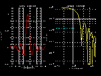
 many of the routines. The first (GRAFTEST.PAS) demonstrates
 the core routines of plotting data and curves with log or
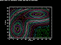
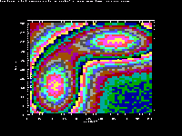
 linear axes. There is a contour plotting demo (CONTEST.PAS)
 that synthesizes some data and plots it in contour plots of
 three different types: contour lines in color, contour lines
 in monochrome, and a "color contour" plot. The other two
 routines demonstrate the cursor (CRSRTEST.PAS) and
 crosshairs (CRHRTEST.PAS) packages in HiGraf.

 First, a couple of words about graphics directories and
 hardware. If the "TPDirectory" compiler directive is defined
 at the top of HIGRAF.PAS, the BGI routines will
 automatically detect the graphics hardware present in your
 machine and load a graphics driver from a directory "C:\TP"
 (this directory is defined in a procedure named
 Initialize_Graph in HiGraf). If the "DefaultDirectory"
 compiler directive is defined, then InitGraph will look for
 the BGI drivers in the default directory.

 If you wish to force the BGI routines to run in a particular
 graphics mode (i.e. the IBM8514 or ATT400 mode on a Compaq)
 or use the AutoMode detect function in InitGraph, choose the
 desired compiler directive to suit your taste.

 The program calling the HiGraf routines must use two data
 types defined in HIGRAF:

 TYPE
   FLOAT = EXTENDED;
   LINLOG = (lin,log);

 These are used in the routines along with more familiar data
 types.

 The basic sequence for using the HiGraf routines is to :

      Initialize_Graph; {sets up hardware}
      Setup_Graph(....); {sets up software variables, etc}
      Axes(...) or Frame(...); {displays axes}
      Label_Axes(...); {labels axes}
      TopTitle(...); {labels the top of the plot}
      XAxisTitle(...) and YAxisTitle(...); {axes labels}
      (do plotting commands: PlotData(...) or PlotPoint(...)
 or
      combinations of Move(...) and Draw(...) or somesuch)
      Then Pause somehow...
      CloseGraph; {BGI closout of graphics}

 That's all there is to it. Take a look at the demo program
 (GRAFTEST.PAS) for more complete details and examples. This
 short example program displays two plots with linear and log
 axes, data points, and other features.

                    

 The following is a listing of the routines in the HIGRAF.PAS
 unit. A couple of definitions are in order first:

 World Coordinates: this coordinate system is the one usually
 used for the plot data; these are FLOAT variables describing
 the data values: i.e. x=1.27,y=1.366E-4, etc.

 Screen Coordinates: these are the INTEGER numbers describing
 the pixel addresses of each pixel; the upper left corner of
 the physical screen is (0,0) in screen coordinates.



              Additional Routines in SCALING.PAS

 Another useful procedure is in SCALING.PAS; often in
 producing plots, you have an array of data (with or without
 error bars) that must be autoscaled. Scale_Axis (in
 SCALING.PAS) takes pointers to these arrays, the type of
 array it is (Byte, Word, etc), the number of values, and the
 type of plot the axis is (Log or Linear). It returns "nice"
 values for the minimum and maximum limits on the axis to be
 plotted and a nice value for the axis labeling interval. One
 way to use it is:

 Scale_Axis(XData,NIL,Byte_Array,100,XWorldMin,XWorldMax,
            XLabelArg,Lin);
 Scale_Axis(YData,NIL,Byte_Array,100,
            YWorldMin,YWorldMax,YLabelArg,Lin
 Setup_Graph(XWorldMin,XWorldMax,YWorldMin,YWorldMax,
             15,90,15,85,Lin,Lin);
 Axes(0,0,XLabelArg/5,YLabelArg/5,5,5,FALSE);
 Frame(XLabelArg/5,YLabelArg/5,5,5,FALSE);
 Label_Axes(XLabelArg,YLabelArg);

 This would give you "nice" axes with 5 minor tick marks
 between axis labels in both X and Y.



            Rapid Contour Plots By Bilinear Patch
         by Neil Judell, Optimal Systems Laboratory,
                        Plainfield, NJ

 In this technique, the points of the original data array are
 viewed as being samples of a function that is continuous,
 with piecewise continuous partial derivatives. This function
 is presumed to be bilinear within the squares delineated by
 the data points. In order to prepare the contour plot of the
 entire region, we merely prepare a contour plot of each
 square "patch" delineated by four adjacent data points.
 There is one potential problem with this method, and that is
 if a contour value is exactly equal to one of the data
 values (one of the values exactly on the corner of a patch),
 then the plot becomes ill-conditioned. In the software
 example provided, this is readily prevented. The data values
 take on only integer values, while the contour levels are
 floating point. We simply prevent any contour value from
 taking on an exact integer value by adding a small number
 (constant called epsilon) if we determine that the contour
 value is an exact integer.

 Once this conditioning problem is resolved, it may readily
 be seen that within a single patch, for a specified contour
 level, exactly three possibilities exist:  no contour line
 crosses the patch, determined if the contour level is either
 less than the minimum of the four corner values or greater
 than the maximum of the corner values; one contour line
 crosses the patch; or two contour lines cross the patch. In
 the case where one contour line crosses the patch, the
 bilinear equation is solved for the endpoints of the contour
 line and the line is plotted.  In the case where two contour
 lines cross the patch, we determine the four endpoints, and
 then must decide which pairs of endpoints to match to draw
 the appropriate contour lines. Define the bilinear
 coefficients for the patch in a coordinate system local to
 the patch, so that the x value ranges from 0 to 1 and the y
 value ranges from 0 to 1, and let the bilinear equation be:

      value(x,y) = ax + by + cxy +d.

 If we now attempt to parametrize the contour line in x in
 terms of y we find:

      x = (value - contour level - by - d)/(a + cy).

 We then see, that because of the nature of the local
 coordinate system, one of the contour lines must have the y
 value of both of its endpoints greater than -a/c, and the
 other contour line must have both of its endpoints less than
 -a/c. (It should be noted that because of the non-integral
 nature of the contour level, we cannot have two contour
 lines in a patch when c=0). This means that if we simply
 sort the four endpoints in increasing value of their y-
 values, that the two endpoints with the lowest y-values form
 a pair for one contour line and the two endpoints with the
 highest y-values form a pair for the other contour line.

 In the software example provided, contour lines are
 approximated by drawing straight lines from one edge of the
 bilinear patch to the other. In cases where the number of
 data points are large relative to the screen pixel density
 (say 20 x 20 data points for an EGA display), this is
 adequate for reasonable contour plots. If the data are
 sparse, it may be desirable to plot the contour line more
 accurately within the patch, using the parametrized equation
 above.

 The software example provided contains the definitions used
 for the contour plotting software, and the pointers to the
 data array and the contour level array. The procedure for
 allocating memory to
 these arrays must be user provided. The data array pointer
 is called data_array_pointer, which points to longint data
 points, via:

       data=data_array_pointer^[x]^[y],

 with 1<=x<max_x_size and 1<=y<max_y_size. The contour level
 array points to type float , and is accessed via:  contour
 level = contours[i], with 1<=i<max_contours.

 The only procedure available for external calling is
 Contour_Plot, which performs the entire plot function.

 The test program, CONTEST.PAS, is a skeleton of a general
 user program employing the contour plot modules. It performs
 the operations minimally necessary for operation. First, it
 allocates storage. Then, it fills the data array.  In this
 example, the data array consists of a sum of two two-
 dimensional Gaussians plus noise. The contour level array is
 then filled with values (which should be in ascending
 order). Initialize_Graph is called to set the display to
 graphics mode, Contour_Plot is called to perform the plot,
 and finally CloseGraph is called to return the display to
 text mode.